4.8 Linear Regression

Before doing GWAS, we’re going to learn about using linear models in R.

Loading a datset:

##  manufacturer          model               displ            year     
##  Length:234         Length:234         Min.   :1.600   Min.   :1999  
##  Class :character   Class :character   1st Qu.:2.400   1st Qu.:1999  
##  Mode  :character   Mode  :character   Median :3.300   Median :2004  
##                                        Mean   :3.472   Mean   :2004  
##                                        3rd Qu.:4.600   3rd Qu.:2008  
##                                        Max.   :7.000   Max.   :2008  
##       cyl           trans               drv                 cty       
##  Min.   :4.000   Length:234         Length:234         Min.   : 9.00  
##  1st Qu.:4.000   Class :character   Class :character   1st Qu.:14.00  
##  Median :6.000   Mode  :character   Mode  :character   Median :17.00  
##  Mean   :5.889                                         Mean   :16.86  
##  3rd Qu.:8.000                                         3rd Qu.:19.00  
##  Max.   :8.000                                         Max.   :35.00  
##       hwy             fl               class          
##  Min.   :12.00   Length:234         Length:234        
##  1st Qu.:18.00   Class :character   Class :character  
##  Median :24.00   Mode  :character   Mode  :character  
##  Mean   :23.44                                        
##  3rd Qu.:27.00                                        
##  Max.   :44.00

There is now an object in memory called mpg, which is a dataframe with 11 variables.

The mpg of cars in a city and the mpg on the highway are encoded in the columns cty and hwy, respectively.

First, plotting these out:

ggplot(mpg, aes(x = cty, 
                y = hwy)) + 
  xlab("City Mileage (mpg)") + 
  ylab("Highway Mileage (mpg)") +
  geom_point() +
  theme_classic()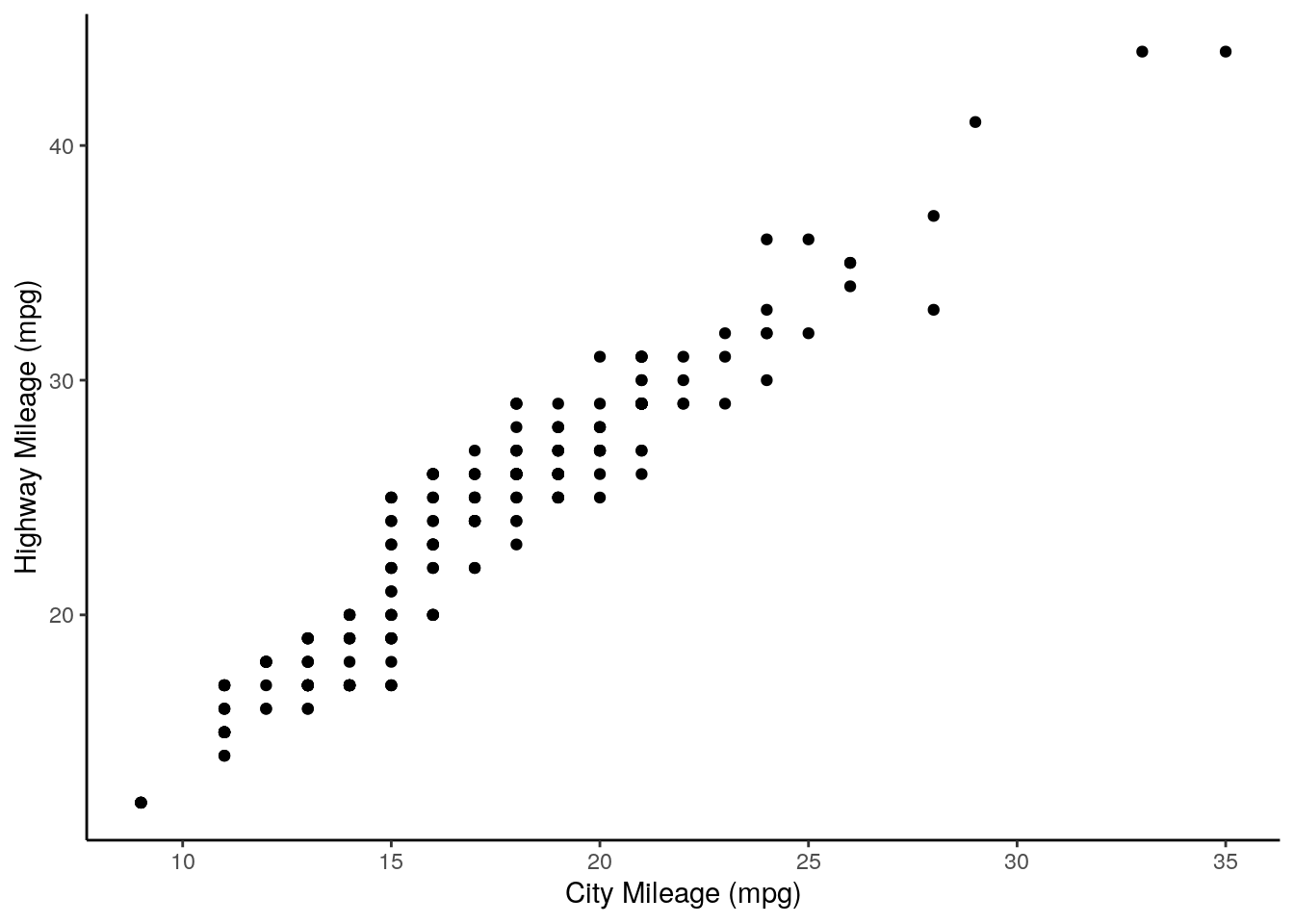

We can use the function lm() to implement a linear model.

lm(formula = hwy ~ cty, data = mpg)

## 
## Call:
## lm(formula = hwy ~ cty, data = mpg)
## 
## Coefficients:
## (Intercept)          cty  
##       0.892        1.337

This first argument, formula is what determines the variables we are regressing, with the tilde (~) sign separating dependent and independent variables. For example, the above formula asks to create a linear model where highway mileage is expressed as a function of city mileage. In other words, we’re doing the good old algebra \[y = mx + b\] except here it’s \[highway = m * city + Intercept\].

We can extract the intercept and coefficient as such:

regression <- lm(formula = hwy ~ cty, data = mpg)
print(regression$coefficients[1])

## (Intercept) 
##   0.8920411

print(regression$coefficients[2])

##      cty 
## 1.337456

Let’s add this to our plot:

ggplot(mpg, aes(x = cty, 
                y = hwy)) + 
  xlab("City Mileage (mpg)") + 
  ylab("Highway Mileage (mpg)") +
  geom_point() +
  theme_classic() +
  geom_abline(slope = regression$coefficients[2], 
              intercept = regression$coefficients[1])

Lastly, let’s get some p values out from this. First, we get a summary of our model:

regression <- lm(formula = hwy ~ cty, data = mpg)
sumRegression <- summary(regression)
print(sumRegression)

## 
## Call:
## lm(formula = hwy ~ cty, data = mpg)
## 
## Residuals:
##     Min      1Q  Median      3Q     Max 
## -5.3408 -1.2790  0.0214  1.0338  4.0461 
## 
## Coefficients:
##             Estimate Std. Error t value Pr(>|t|)    
## (Intercept)  0.89204    0.46895   1.902   0.0584 .  
## cty          1.33746    0.02697  49.585   <2e-16 ***
## ---
## Signif. codes:  0 '***' 0.001 '**' 0.01 '*' 0.05 '.' 0.1 ' ' 1
## 
## Residual standard error: 1.752 on 232 degrees of freedom
## Multiple R-squared:  0.9138, Adjusted R-squared:  0.9134 
## F-statistic:  2459 on 1 and 232 DF,  p-value: < 2.2e-16

From the Coefficients, we want to get the value of Pr(>|t|). We can access Coefficients using the $ operator:

print(sumRegression$coefficients)

##              Estimate Std. Error   t value      Pr(>|t|)
## (Intercept) 0.8920411 0.46894568  1.902227  5.838000e-02
## cty         1.3374556 0.02697315 49.584698 1.868307e-125

And now we can index this to get our p value:

print(sumRegression$coefficients["cty", "Pr(>|t|)"])

## [1] 1.868307e-125

This is a very low p value, reflecting the strongly non-zero slope of our regression line.