3.3 Class 5: Lotka-Volterra I: Competition
To begin with, a simple implementation of the Lotka-Volterra equation in R, with discrete time points:
# Initialize conditions
# Population Sizes
N1 <- 30
N2 <- 20

# Carrying Capacities
K1 <- 1000
K2 <- 400

# Interaction parameters between pops
alpha <- 0.1
beta <- 0.9

# Growth rates
r1 <- 1.5
r2 <- 1.3

# Simulation time
nYears <- 20

# Vectors to store population sizes
n1_list <- c(N1)
n2_list <- c(N2)

# Run simulation
for (i in seq(nYears)){
  # Calculate future pop sizes for next time point
  # Saving N1 as a new variable so that it the current value of N1
  # can be used to calculate N2
  N1_future <- N1 + r1 * N1 * ((K1 - N1 - alpha * N2)/K1)
  N2_future <- N2 + r2 * N2 * ((K2 - N2 - beta * N1)/K2)

  # Update N1 and N2
  N1 <- N1_future
  N2 <- N2_future

  # Save to list
  n1_list <- c(n1_list, N1)
  n2_list <- c(n2_list, N2)
}

# Convert to data frame
df <- data.frame(
  time = seq(length(n1_list)),
  n1 = n1_list,
  n2 = n2_list
)

# Convert to tall format
df <- melt(df, id.vars = "time")
colnames(df) <- c("time", "pop", "size")

# Plot
ggplot(df, aes(x = time,
               y = size,
               color = pop)) +
  geom_line() +
  geom_point() +
  labs(x = "Time (Generations)",
       y = "Population Size",
       color = "Population") +
  theme_bw()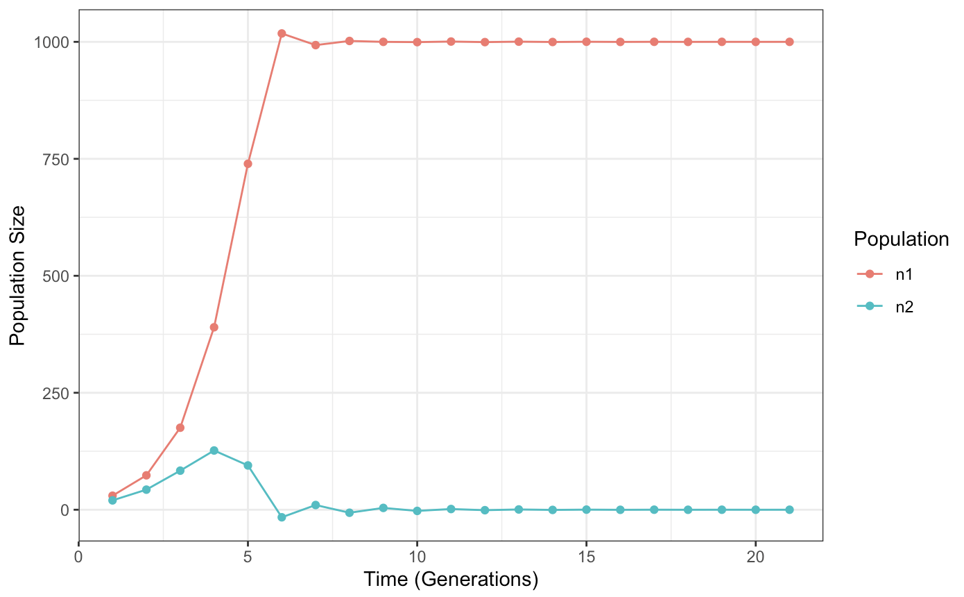
A couple things are apparent from this mode:
- Under these conditions, both populations are not able to coexist - after a brief period of growth, population 2 collapses to 0.
- In this model, population 2 dips below 0 at generation 6.
The first behavior is fine - it’s a pretty basic property of this model that many parameter combinations lead to one population outcompeting the other to extinction. This is called competitive exclusion.
The second behavior - dipping below zero - is not desirable. While our models are theoretical representations of reality, unrealistic behaviors like this are good to correct.
Here, shooting below zero happens because with a large step size and a large growth rate, our model moves too quickly. In response to this, we can decrease our step size. In fact, if we decrease our step size enough, our model very closely approximates the continuous form of the equation.
# Initialize conditions
# Population Sizes
N1 <- 30
N2 <- 20

# Carrying Capacities
K1 <- 1000
K2 <- 400

# Interaction parameters between pops
alpha <- 0.1
beta <- 0.9

# Growth rates
r1 <- 1.5
r2 <- 1.3

# Simulation time
nYears <- 20

# Vectors to store population sizes
n1_list <- c(N1)
n2_list <- c(N2)

# Create a step size
stepSize <- 0.01

# Run simulation
for (i in seq(nYears/stepSize)){   # Scale our for loop range by the step size
  # Calculate future pop sizes for next time point
  # Saving N1 as a new variable so that it the current value of N1
  # can be used to calculate N2
  N1_future <- N1 + r1 * N1 * ((K1 - N1 - alpha * N2)/K1) * stepSize # Multiply by step size
  N2_future <- N2 + r2 * N2 * ((K2 - N2 - beta * N1)/K2)  * stepSize # Multiply by step size

  # Update N1 and N2
  N1 <- N1_future
  N2 <- N2_future

  # Save to list
  n1_list <- c(n1_list, N1)
  n2_list <- c(n2_list, N2)
}

# Convert to data frame
df <- data.frame(
  time = seq(length(n1_list)),
  n1 = n1_list,
  n2 = n2_list
)

# Convert to tall format
df <- melt(df, id.vars = "time")
colnames(df) <- c("time", "pop", "size")

# Plot
ggplot(df, aes(x = time * stepSize, # We multiply time by stepSize to convert back to years
               y = size,
               color = pop)) +
  geom_line() +
  labs(x = "Time (Generations)",
       y = "Population Size",
       color = "Population") +
  theme_bw()
A few changes are needed to make this work:
- The for loop is changed to incorporate step size:
for (i in seq(nYears/stepSize)). If, previously, each step represented one generation, each step now represents one generation * stepSize - just a fraction of the time. In other words, we need to run our model more times to represent an equal amount of real time. - When calculating population sizes, we incorporate step size:
N1_future <- N1 + r1 * N1 * ((K1 - N1 - alpha * N2)/K1) * stepSize - Lastly, when plotting, we convert time back to years by multiplying by stepSize again:
ggplot(df, aes(x = time * stepSize,
So far, we have seen models where one population outcompetes the other. It is worth noting that this is not an inherent property of Lotka-Volterra models:
# Initialize conditions
# Population Sizes
N1 <- 30
N2 <- 20

# Carrying Capacities
K1 <- 1000
K2 <- 1000

# Interaction parameters between pops
alpha <- 0.4
beta <- 0.9

# Growth rates
r1 <- 1.5
r2 <- 1.3

# Simulation time
nYears <- 20

# Vectors to store population sizes
n1_list <- c(N1)
n2_list <- c(N2)

# Create a step size
stepSize <- 0.01

# Run simulation
for (i in seq(nYears/stepSize)){ # Scale our for loop range by the step size
  # Calculate future pop sizes for next time point
  # Saving N1 as a new variable so that it the current value of N1
  # can be used to calculate N2
  N1_future <- N1 + r1 * N1 * ((K1 - N1 - alpha * N2)/K1) * stepSize # Multiply by step size
  N2_future <- N2 + r2 * N2 * ((K2 - N2 - beta * N1)/K2) * stepSize # Multiply by step size

  # Update N1 and N2
  N1 <- N1_future
  N2 <- N2_future

  # Save to list
  n1_list <- c(n1_list, N1)
  n2_list <- c(n2_list, N2)
}

# Convert to data frame
df <- data.frame(
  time = seq(length(n1_list)),
  n1 = n1_list,
  n2 = n2_list
)

# Convert to tall format
df <- melt(df, id.vars = "time")
colnames(df) <- c("time", "pop", "size")

# Plot
ggplot(df, aes(x = time / stepSize, # We multiply time by stepSize to convert back to years
               y = size,
               color = pop)) +
  geom_line() +
  labs(x = "Time (Generations)",
       y = "Population Size",
       color = "Population") +
  theme_bw()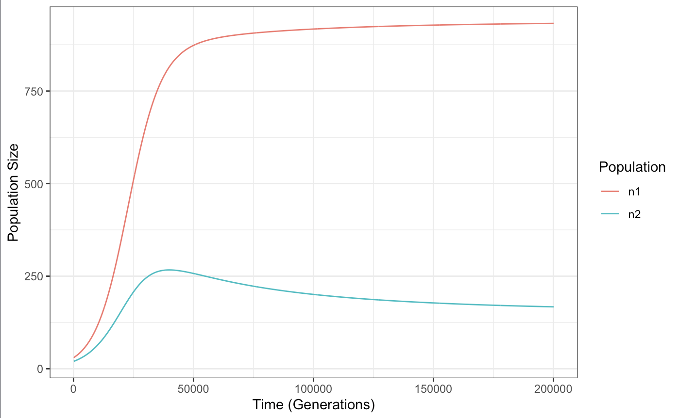
Note that when both populations coexist, they do not hit their carrying capacities:
# Initialize conditions
# Population Sizes
N1 <- 30
N2 <- 20

# Carrying Capacities
K1 <- 1000
K2 <- 900

# Interaction parameters between pops
alpha <- 0.4
beta <- 0.9

# Growth rates
r1 <- 1.5
r2 <- 1.3

# Simulation time
nYears <- 20

# Vectors to store population sizes
n1_list <- c(N1)
n2_list <- c(N2)

# Initialize variables to store population size for the logistic model
# We start at the same point as the LV model
N1_logistic <- N1
N2_logistic <- N2

# Lists to store
n1_list_logistic <- c(N1_logistic)
n2_list_logistic <- c(N2_logistic)

# StepSize
stepSize <- 0.01

for (i in seq(nYears/stepSize)){
  # Calculate LV dynamics
  N1_future <- N1 + r1 * N1 * ((K1 - N1 - alpha * N2)/K1) * stepSize
  N2_future <- N2 + r2 * N2 * ((K2 - N2 - beta * N1)/K2) * stepSize

  # Update N1 and N2
  N1 <- N1_future
  N2 <- N2_future

  # Save to list
  n1_list <- c(n1_list, N1)
  n2_list <- c(n2_list, N2)

  # Calculate logistic dynamics
  N1_logistic <- N1_logistic + r1 * (1 - N1_logistic/K1) * N1 * stepSize
  N2_logistic <- N2_logistic + r2 * (1 - N2_logistic/K2) * N2 * stepSize

  # Save to list
  n1_list_logistic <- c(n1_list_logistic, N1_logistic)
  n2_list_logistic <- c(n2_list_logistic, N2_logistic)
}

# Store LV data as a data frame
df <- data.frame(
  time = seq(length(n1_list)),
  n1 = n1_list,
  n2 = n2_list
)

# Reorganize to a tall dataframe
df <- melt(df, id.vars = "time")
colnames(df) <- c("time", "pop", "size")
# Add a column with the model name
df["Model"] = "Lotka-Volterra"

# Store Logistic data as a data frame
df_logistic <- data.frame(
  time = seq(length(n1_list_logistic)),
  n1 = n1_list_logistic,
  n2 = n2_list_logistic
)

# Reorganize to a tall dataframe
df_logistic <- melt(df_logistic, id.vars = "time")
colnames(df_logistic) <- c("time", "pop", "size")
# Add a column with the model name
df_logistic["Model"] = "Logistic"

# Combine LV and logistic dataframes into one for plotting
df_plot <- rbind(df, df_logistic)

# Reorganize the factor levels of our plotting data
# This determines which population is plotted in dotted lines
df_plot$Model <- factor(df_plot$Model,
                      levels = c("Lotka-Volterra", "Logistic"))

ggplot(df_plot, aes(x = time / stepSize,
                    y = size,
                    color = pop,
                    linetype = Model)) +
  geom_line() +
  labs(x = "Time (Generations)",
       y = "Population Size",
       color = "Population") +
  theme_bw()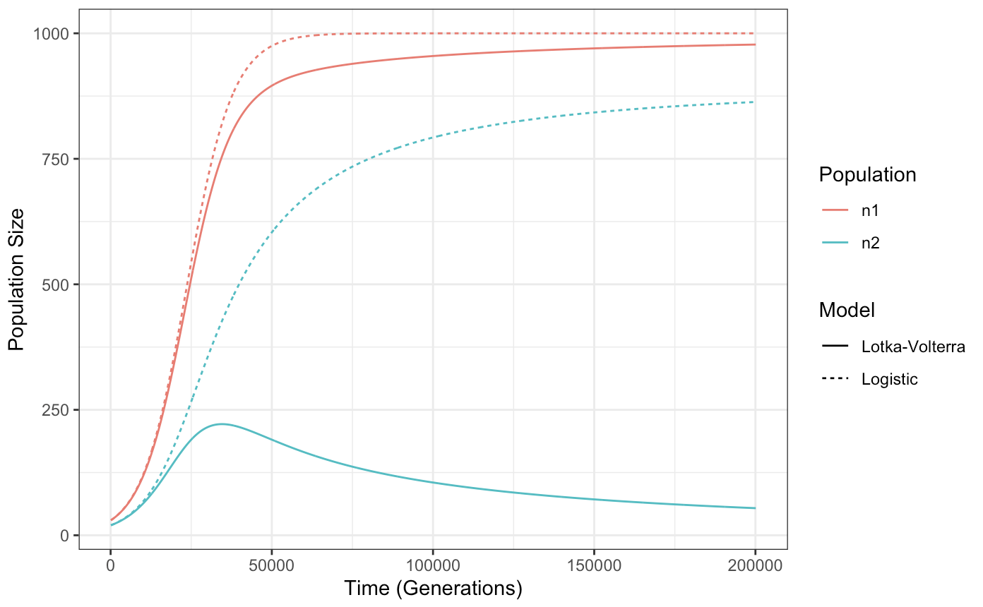
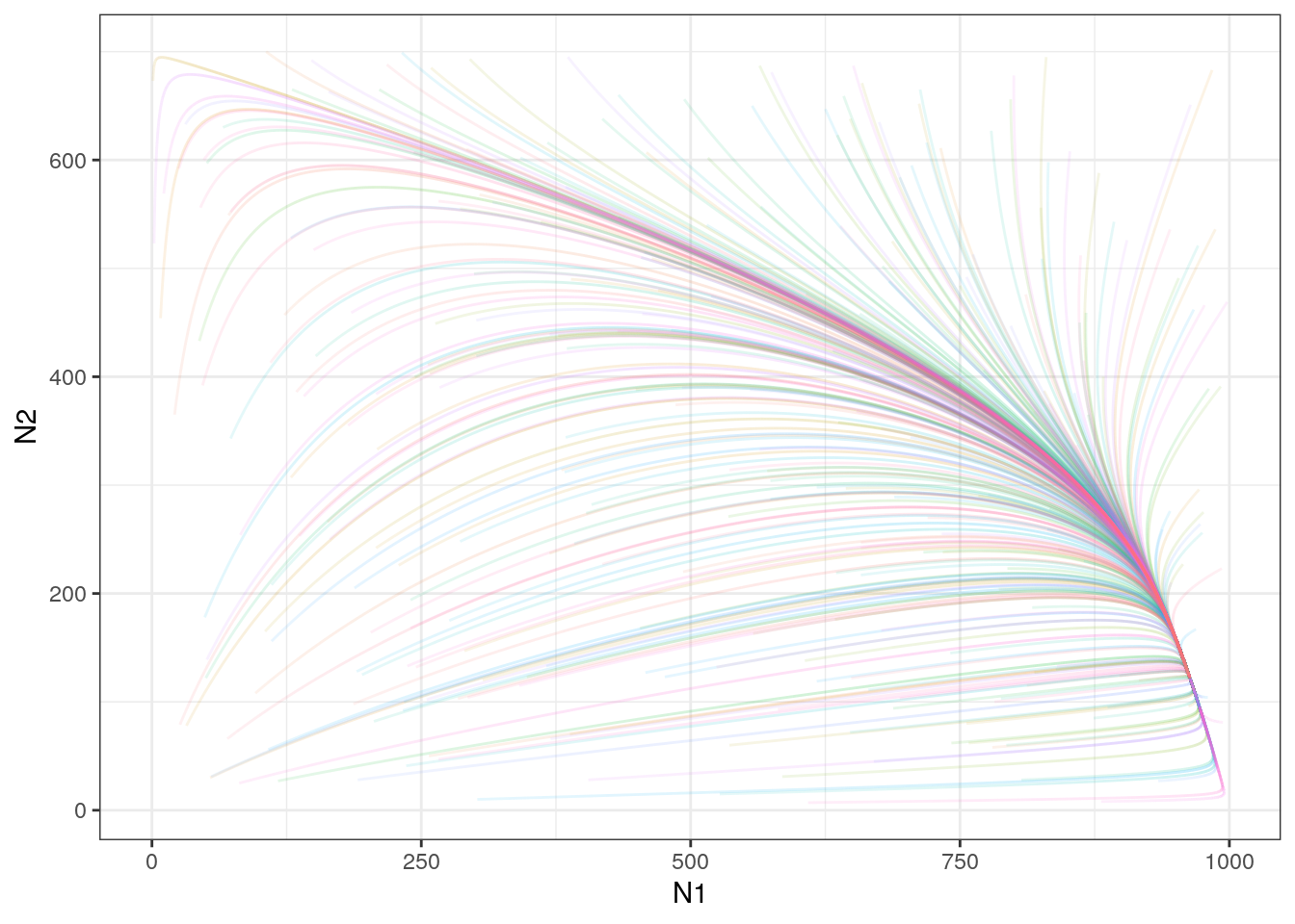
3.3.1 Equilibirum from multiple starting points
Now, starting from multiple conditions:
# Initialize conditions
# Carrying Capacities
K1 <- 1000
K2 <- 700

# Interaction parameters between pops
alpha <- 0.3
beta <- 0.6

# Growth Rates
r1 <- 1.5
r2 <- 1.3

# Length of population
nYears <- 20


# Lists to store population sizes, trial numbers, and time within each trial
n1_all_trials <- c()
n2_all_trials <- c()
trialNumber <- c()
time <- c()

# Step Size
step <- 0.01

# Number of trials we are running
nTrials <- 300

# Run simulation
for (trial in seq(nTrials)){
  # Randomly generate starting population sizes
  N1 <- sample(seq(K1), 1)
  N2 <- sample(seq(K2), 1)

  # Create a list for population sizes
  n1_list <- c(N1)
  n2_list <- c(N2)

  # Run the simulation
  for (i in seq(nYears/step)){
    # Calculate population size
    N1_future <- N1 + r1 * N1 * ((K1 - N1 - alpha * N2)/K1) * step
    N2_future <- N2 + r2 * N2 * ((K2 - N2 - beta * N1)/K2) * step

    N1 <- N1_future
    N2 <- N2_future

    # Add to lists
    n1_list <- c(n1_list, N1)
    n2_list <- c(n2_list, N2)
  }

  # Add simulation results to overall results
  n1_all_trials <- c(n1_all_trials, n1_list)
  n2_all_trials <- c(n2_all_trials, n2_list)
  trialNumber <- c(trialNumber, rep(trial, time = length(n1_list)))
  time <- c(time, seq(length(n1_list)))
}

# Store as data frame
df <- data.frame(
  n1 = n1_all_trials,
  n2 = n2_all_trials,
  trial = trialNumber,
  time = time
)

# Plot
ggplot(df, aes(x = n1,
               y = n2,
               color = factor(trial), # Factor lets R know that trial is a category, not a continuous number
               alpha = time)) + # Transparency is controlled by time within trial - dark points are the last times within a trial
  geom_path() +
  guides(color="none",
         alpha = "none") + # Remove color and transparency scales
  xlab("N1") +
  ylab("N2") +
  theme_bw()